STORY OF THE MONTH
Ten Thousand Spins, Seventeen Chips
 Sep 2026
  Vaisakh Mannalath
The ten-thousand-spin challenge
At the end of a narrow street stood a casino with no roulette wheel and no card tables. Its only game was an electronic machine called The Ten-Thousand-Spin Jackpot.
A mathematician bought one ticket. The ticket started a rapid batch of $10{,}000$ electronic spins, completed in seconds.
Each spin produced either a rare gold star or a blank. A visible state meter changed after every result. The new state could raise or lower the probability of a gold symbol on the next spin. Consequently, the next probability could depend on the complete sequence of earlier outcomes.
Two counters
Before spin i, the machine calculated the conditional probability pi of producing a gold symbol. It added pi to a probability counter and then performed the spin. The result entered a separate concealed counter.
The machine repeats the same sequence—record the probability, spin, hide the result—ten thousand times.
When the batch ended, the House added the $10{,}000$ recorded probabilities. It revealed
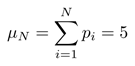
but kept the actual number of gold symbols sealed.
The number 5 described the accumulated chance across the changing spins. The actual gold-symbol count remained unknown.
The House gave the mathematician a board numbered from 0 to 10,000. To submit a range, the mathematician had to place one chip on every count it contained. If the sealed count was covered, the wager earned a fixed prize; otherwise it lost. The mathematician therefore sought a highly reliable range requiring as few chips as possible.
Applying two mathematical tools
The mathematician knew several concentration inequalities for constructing such ranges (1, 2). They applied each method at the same 99% coverage level, corresponding to the failure allowance

The same coverage level makes the two ranges directly comparable.
First tool: Azuma–Hoeffding
The mathematician first applied the standard Azuma–Hoeffding bound. It remains valid even when later probabilities depend on earlier outcomes (1, 3). Its generality, however, comes with a substantial cost in a rare-event game: it only uses the facts that there are 10,000 trials and that every spin contributes either zero or one gold symbol.
For

the Azuma–Hoeffding wager was
0-167 gold symbols
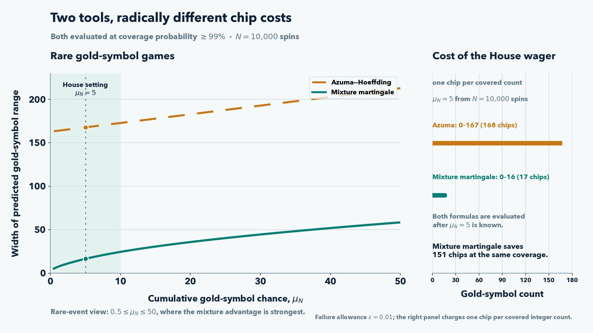
This interval admitted 168 possible integer counts, so the mathematician needed 168 chips. It was valid, but extremely broad relative to a cumulative gold-symbol chance of five. The interval was calculated using the two-sided construction described in Ref. 3.
Second tool: a mixture martingale
The mathematician then applied a mixture-martingale bound. Instead of relying on one statistical tuning, this rule combined a predetermined range of tunings into one valid test (2, 3).
For exactly the same hidden game and the same 99% promise, the mixture-martingale wager was
0-16 gold symbols
Only 17 possible integer counts remained, so this wager required 17 chips. The mixture martingale therefore saved 151 chips relative to Azuma–Hoeffding—a reduction of approximately 90% in the number of covered counts. The 90% figure refers specifically to interval size.
The interval sizes settle the comparison.
The game mathematically
Let Xi=1 when spin i produces a gold symbol and Xi=0 otherwise. The hidden count and revealed cumulative conditional probability are
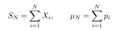
The statistical rule constructs L and U satisfying

Half of the failure budget protects each end of the two-sided interval. The probabilities may change with the entire history, yet the coverage statement remains valid.
| Registered rule | Covered counts | Chips required |
| Azuma–Hoeffding | 0–167 | 168 |
| Mixture martingale | 0–16 | 17 |
Why the difference becomes large
Azuma–Hoeffding pays for the possibility of fluctuations across all 10,000 bounded trials. The mixture martingale can use the fact that the cumulative conditional probability is only five. The distinction becomes pronounced when the event of interest is rare.
The following animation shows the exact interval widths for rare-event games with the same N=10,000 and epsilon=0.01. The House setting Un=5 is highlighted.
The plotted window isolates the rare-event regime $0.5\le\mu_N\le50$, where the advantage is strongest.
From the casino to QKD
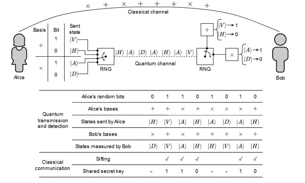
The jackpot game reproduces the statistical structure encountered in QKD. Quantum key distribution produces long sequences in which useful detections or errors can be rare. The probability of a later event may also depend on the earlier record. Security proofs must nevertheless convert finite observations into rigorous statements about quantities that may not be directly observed (3, 4).
Satellite QKD can provide a long-distance backbone connecting terrestrial segments of future quantum networks (5, 6). During each satellite pass, only a small fraction of the transmitted optical pulses may produce useful detections. The link changes with elevation, diffraction, atmospheric propagation, pointing, tracking and background conditions, producing a finite, sparse and non-stationary record (3, 4, 5). As these satellite links are combined with terrestrial links and network-routing operations, the resulting detection and error records can also become non-identically distributed and history dependent (6, 7).
A finite-key security proof must convert these records into bounds on quantities such as single-photon detections and phase errors (3, 4). Sharper mixture-martingale bounds preserve more of the available information, improving the statistical foundation for satellite links and the wider quantum networks they connect.
That is the lesson of the House of Changing Odds. With the right mathematics, even changing odds and rare events yield precise statistical conclusions.
References
- K. Azuma, “Weighted sums of certain dependent random variables,” Tohoku Mathematical Journal 19, 357–367 (1967). doi:10.2748/tmj/1178243286
- E. Kaufmann and W. M. Koolen, “Mixture Martingales Revisited with Applications to Sequential Tests and Confidence Intervals,” Journal of Machine Learning Research 22, 1–44 (2021). Open article
- V. Mannalath, V. Zapatero, K. Tamaki and M. Curty, “Quantum Key Distribution Beyond Stationary Channels” (2026). arXiv:2607.17690
- J. S. Sidhu et al., “Finite key effects in satellite quantum key distribution,” npj Quantum Information 8, 18 (2022). doi:10.1038/s41534-022-00525-3
- S.-K. Liao et al., “Satellite-to-ground quantum key distribution,” Nature 549, 43–47 (2017). doi:10.1038/nature23655
- Y.-A. Chen et al., “An integrated space-to-ground quantum communication network over 4,600 kilometres,” Nature 589, 214–219 (2021). doi:10.1038/s41586-020-03093-8
- M. Pant et al., “Routing entanglement in the quantum internet,” npj Quantum Information 5, 25 (2019). doi:10.1038/s41534-019-0139-x
OTHER STORIES